(Tips) パワースペクトルの波数・周波数分布の作り方
作成者: 西本絵梨子
編集履歴
- 2014年2月14日: 新規作成。
- 2014年2月28日: GPhys::FFTのコマンドをさらに活用する方法について追記。
- 2014年3月17日: データの前処理(特定の周期を除去)についてのサンプルプログラムを追加。
- 2014年6月 3日: パワースペクトル密度の定義を一般的なものに変更。それに伴い、wavenum_freq.rbとwavenum_freq_2.rbを変更。
概要
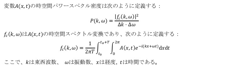
熱帯OLRのパワースペクトルを計算して、波数・周波数空間でのパワースペクトル分布を描くサンプルプログラムです。 Wheeler and Kiladis (1999) JASの図1のようなものを描きます。
計算手順
1980年1月から2010年12月までのNOAA/OLR日平均データを使用。 データは次のサイトから入手できる:NOAA/OLR
- あらかじめ、365日、182.5日、122日の周期成分をデータから除去しておく。 (サンプルプログラム:remove_AC.rb)
赤道対称・反対称分離操作をほどこす。
赤道対称成分: OLRsym=(OLR(x,y,t)+OLR(x,-y,t))/2.0
赤道反対称成分: OLRasym=(OLR(x,y,t)-OLR(x,-y,t))/2.0
- GPhys::FFTをつかって、月ごとにフーリエ変換を経度・時間方向にほどこし、パワースペクトルを得る。このとき、その月のデータとして月開始の30日前から92日分のデータを使用する。
- 各月のパワースペクトルを足し合わして平均する。(平滑化)
- 東進成分と西進成分に分ける。k>0として、w>0が西進、w<0が東進。
- x(i) (i=0,1,..,N-1)のFFTの結果には、i=0,1,...,[N/2-1]まではx(i)のフーリエ変換X(i)が入っているが、残りi=N/2,..N-1にはX(N-i+1)が入っている。
- GPhys::FFTだと、時間方向のFFT成分の、前半分は西進成分が入っていて、後半分には東進成分が後ろから入っていると考えればよい。
ダウンロード
ソースコード
サンプル2
#
# draw the wavenumber-frequency diagram
# like Fig.1 of Wheeler and Kiladis [1999] JAS
# using GPhys::FFT
#
#-- create: 28 Feb. 2014 Eriko Nishimoto
#-- modified: 03 Jun. 2014 Eriko Nishimoto
#
require "numru/ggraph"
include NumRu
pi=Math::PI
type="sym"
type="antisym"
#-----------------------------settings
monlist=NArray.int(12).indgen(1,1)
#yrlist=NArray.int(30).indgen+1980
yrlist=NArray.int(5).indgen+1980
nperiod=92
#-----------------------------open data
#-- daily OLR data removed the cycles of 365days, 182.5days, 122days
dir="/raid/sup1/data/NOAAOLR/FFT/NetCDF/"
fname="daily_rmAC.nc"
var="olr_detrend"
slat, elat=-15, 15
dum=GPhys::IO.open(dir+fname,var).cut(true,slat..elat,true)
#-----------------------------make data
#-- components of antisymmetric and symmetric about the equator
nx,ny,nt=dum.shape
mask=NArray.int(ny).indgen(-1,-1)+ny
if type=="sym"
#-----------------------------symmetric component
#-- (a(x,y,t)+a(x,-y,t))/2
tmp=(dum+dum[true,mask,true])/2.0
figtitle="LOG10{ POWER(OLR S) }"
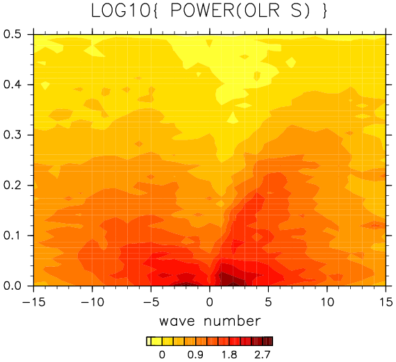
elsif type=="antisym"
#-----------------------------antisymmetric component
#-- (a(x,y,t)-a(x,-y,t))/2
tmp=(dum-dum[true,mask,true])/2.0
figtitle="LOG10{ POWER(OLR A) }"
end
#-----------------------------FFT
nx=tmp.shape[0]
nx_2,nt_2=nx/2,nperiod/2
ps=NArray.float(nx,nperiod).fill(0)
fc=[]
yrlist.each{|yr|
monlist.each{|mn|
#----------------------use data of nperiod
st=Date.parse("#{yr}-#{mn}-01")-30
et=st+nperiod-1
data=tmp.cut(false,st..et)
nx,ny,nt=data.shape
#----------------------foward FFT
GPhys::fft_ignore_missing(true)
fc=data.fft(false,0,2).mean(1)
#----------------------change axes
z0=fc.axis(0).pos
fc.axis(0).set_pos(-z0)
z1=fc.axis(-1).pos.convert_units("day-1")/(2.0*pi)
fc.axis(-1).set_pos(z1)
#----------------------power spectral
#-- |fc|^2
power=(fc.abs**2).val
ps+=power/monlist.length/yrlist.length
}
}
power=fc.copy.replace_val(ps).rawspect2powerspect(0,-1)\
.spect_zero_centering(0).spect_one_sided(-1)
p power.units
#====================================draw
#--settings
colormap = 8
psname = "Fig/"+$0.split('.')[0]+"_#{type}"
p psname
#--
DCL.sgscmn(colormap)
DCL.swcset 'fname',psname
iws = (ARGV[0]||(puts 'Workstation ID(I)?'; DCL.sgpwsn; gets)).to_i
DCL.gropn iws
DCLExt.sg_set_params 'lcntl'=>false
DCLExt.uz_set_params 'indext1'=>3,'indext2'=>5\
,'indexl1'=>5,'indexl2'=>5,'inner'=>-1
GGraph.set_fig "viewport"=>[0.08,0.92,0.2,0.8]
GGraph.set_axes "xunits"=>"","yunits"=>""\
,"xtitle"=>"wave number","ytitle"=>"frequency (1/day)"
GGraph.tone power.log10.cut(-15..15,0..0.5),true\
,"annot"=>false,"title"=>figtitle
GGraph.color_bar "landscape"=>true
DCL.grcls
参考文献
- Wheeler, M., and G. N. Kiladis, 1999: Convectively Coupled Equatorial Waves: Analysis of Clouds and Temperature in the Wavenumber--Frequency Domain. J. Atmos. Sci., 56, 374-399.
- 林良一, 1980: 最近の時空間スペクトル解析法の発展と大気大規模波動への応用. 天気, 27, 3-21.
キーワード:[FFT]
参照:[(Tips) パワースペクトルの波数・周波数分布(2)]